Performance Portability of Do Concurrent in Fortran
Table of Contents
So you have a Fortran application and you want to make it use GPUs without having to:
- rewrite your codebase
- replicate the code and have separate CPU and GPU implementations
Although they sound simple being able to fulfill these two requirements is extremely complicated. This brief writeup is a summary of my recent experiences in porting Fortran code to use GPUs.
I will assume that you are already familiar with GPUs and you’re interested in learning other pathways to get an application to use GPUs with performance and portability in mind.
The many ways to GPU#
All roads lead to Rome, or so they say. There are multiple pathways to use GPUs in the current time. There are the explicit programming languages you can use to access GPUs, such as: CUDA from NVIDIA, HIP/ROCM from AMD, OpenCL from OpenCL, and Sycl from Intel. These models rely on the developer writing code using the proprietary or open source runtimes the vendors provide in the form of an Application Programming Interface (API). Using these models, one can extract as much performance as possible from the hardware - however, the barrier height to overcome to be able to do so is rather high.
Another option is to use directives, which involves adding decorators around your code to tell the compiler to generate code that will use GPUs. The options here are OpenMP and OpenACC. They all have a standards committee and promise portability, i.e. code accelerated with it should run on any vendor’s hardware. However, they have the disadvantage that the portability and the performance is 100% up to the compiler. Therefore, it is quite simple to get good performance out of the hardware if the implementation in the compiler is solid - thus, the barrier height to overcome to get code on GPUs using directives is much lower than with CUDA, HIP, or SYCL.
Now there is a third option, specifically in Fortran, which is the use of standard parallelism. Fortran introduced the do concurrent construct in Fortran 2008 and it indicates to the compiler that the iterations of the loop are independent between each other and that the code in the loop has no side effects whatsoever. The goal was to help the compiler detect simple optimizations that it could perform to vectorize the code in the loop. Additionally, with the existence of OpenMP and OpenACC it was a prime construct to be exploited by threading models. Most compilers will map a do concurrent loop into whatever parallelism backend they prefer. For example, the NVIDIA compiler maps it to OpenACC, while the AMDFlang compiler maps it to OpenMP, as does the Intel compilers.
All three major vendors have released compiler support for do concurrent loops onto their hardware, making it an attractive pathway to obtain portable GPU performance.
Do concurrent and memory transfers#
If you’ve done any type of GPU programming you’re aware that they live in separate memory address spaces. The host (CPU) and the device (GPU) are connected via an interconnect - sometimes PCIe or a proprietary one depending on the hardware vendor.
In the early days of GPU programming it was up to the user to transfer data in between the host and the device. This was/is one of the most complex tasks of GPU programming. Since the interconnect is limited by the bandwidth and latency, the transfer of data between host and device can quickly become a bottleneck. Newer versions of the runtimes are able to deduce at runtime if a pointer is on the host or the device and transfer it automatically to wherever it is needed. This is very nice indeed, however it can have severe performance penalties since an array that could be transferred once might be transferred back and forth whenever it is used in the host or device.
Therefore, for good performance it is up to the user to transfer data between the host and the device. Since we’ve decided to adopt do concurrent as our method for parallelization we will use another “directive” base approach to handle our memory. We will use OpenMP since it is what I am most familiar with.
The most useful directives for us will be:
!$omp target enter data map(to/alloc: )
!$omp target exit data map(from/release/delete:)
!$omp target update to/from()
OpenMP creates target regions which are areas (scope) where statements can be executed on the GPU. For example:
!$omp target
a = b + c
!$omp end target
This operation will take place on the GPU. OpenMP works similar to using it for parallelism on the CPU:
!$omp target teams loop
do i = 1, n
c(i) = alpha * a(i) + b(i)
end do
That will be executed on the GPU, the runtime is smart enough to know that it needs to transfer the arrays and the constant to the GPU. However, you can be more detailed and use:
!$omp target teams loop map(to: a,b) map(tofrom: c)
do i = 1, n
c(i) = alpha * a(i) + b(i)
end do
This now allows you to tell the compiler that you do not need a or b copied back, you’ve now deleted two unnecessary copies that needed to happen. With do concurrent you cannot do this specifically…the original loop would simply look like:
do concurrent(i=1:n)
c(i) = alpha * a(i) + b(i)
end do
But since do concurrent is part of the Fortran language, it does not have directives that you can add around it to reduce the amount of copies. So you’ll have to resort to OpenMP. You can do:
!$omp target data
!$omp target update to(a,b,c)
do concurrent(i=1:n)
c(i) = alpha * a(i) + b(i)
end do
!$omp target update from(c)
!$omp end target data
With the target data region I can select the scope through which the data will be “alive” for the CPU/GPU boundary. The moment we leave the target region the pointers get deleted.
However, you might wonder what if I want a variable to live in the GPU for the duration of my entire program. That’s something very important, specially since for best performance you want to make sure that data needs to be transferred as little a possible between the host and the device. Declaring multiple target regions can be complex. To do this, you can use the omp target enter data map directive.
!$omp target enter data map(to: a,b,c)
do concurrent(i=1:n)
c(i) = alpha * a(i) + b(i)
end do
!$omp target exit data map(from: c)
!$omp target exit data map(delete: a,b,c)
With the enter data clause, the pointer to that spot in memory will be alive as long as you don’t delete it. Careful for memory leaks!
The next question you might ask yourself: why do I need to transfer a and b from the host to the device? Can I just initialize them all on the device and then just copy the resulting array back? Well, yes, you can do that.
!$omp target enter data map(alloc: a,b,c)

! initialize
do concurrent(i=1:n)
c(i) = 0.0
a(i) = 2.0
b(i) = 17.0
end do

do concurrent(i=1:n)
c(i) = alpha * a(i) + b(i)
end do

!$omp target exit data map(from: c)
!$omp target exit data map(delete: a,b,c)
Very nice! now there’s no time wasted with initializing on the host and transferring. We went from having to do 6 total transfers to just 1. You might ask now, in Fortran we can do things like
c = 0.0
! or
c(:) = 0.0
Yes, but those don’t get very well optimized for the GPU if you use them. Use do concurrent for the device. This is the first problem, since if you want to do things on the host you’d probably like to use the array like operations, since they vectorize quite well. So maybe you can write a function that is something similar to:
subroutine initialize_array(array,value,  device)
real(dp), intent(inout) :: array(:)
real(dp), intent(in) :: value
logical, optional, intent(in) :: device

if(device .and. size(array,1) > threshold) then
	do concurrent(i=1:size(array,1))
		array(i) = value
	end do
else
	array = value
end if

end subroutine initialize_array
However, do concurrent should vectorize quite well too. TODO measure this.
Performance#
Our big interest is indeed making sure we get the most out of our code. Do concurrent is very nice in this regard, it maps quite well and vectorizes and optimizes. However, there are work distribution topics we need to think about whenever we want to parallelize something on the GPU. We know that Fortran is column major, versus C is row major. Thus, the loop:
do i = 1, ni
	do j  = 1, nj
		A(i,j) = B(i,j)
	end do
end do
Will perform worse than if we traverse first over j and then over i, on the CPU. You will see the effect of this at larger sizes. This will get worse if you’re looping over higher dimensional arrays, say a 3d array. All of this was inspired from a loop that looks similar to this:
     do concurrent (j=1:ny, i=1:nx)
        if (mask(i,j) <= 0.0_real64) cycle
        do k = 2, nz-1
           a_loc   = a3d(i,j,k)
           h_loc   = h3d(i,j,k)
           ray_loc = ray(i,j)
           b1_loc  = b1(i,j)
           d1_loc  = d1(i,j)

           c1(i,j,k) = dt * a_loc * b1_loc

           b_denom = h_loc + dt * (ray_loc + a_loc * d1_loc)
           b1_loc  = one / (b_denom + dt * a3d(i,j,k+1))
           d1_loc  = b_denom * b1_loc

           u_prev  = unew(i,j,k-1)
           u_loc   = (h_loc * u(i,j,k) + dt * a_loc * u_prev) * b1_loc
           unew(i,j,k) = u_loc

           b1(i,j) = b1_loc
           d1(i,j) = d1_loc
        end do
     end do
This loop can be conveniently rewritten further using do concurrent’s features:
     do concurrent (j=1:ny, i=1:nx, mask(i,j) >= 0.0_real64)
        do k = 2, nz-1
           a_loc   = a3d(i,j,k)
           h_loc   = h3d(i,j,k)
           ray_loc = ray(i,j)
           b1_loc  = b1(i,j)
           d1_loc  = d1(i,j)

           c1(i,j,k) = dt * a_loc * b1_loc

           b_denom = h_loc + dt * (ray_loc + a_loc * d1_loc)
           b1_loc  = one / (b_denom + dt * a3d(i,j,k+1))
           d1_loc  = b_denom * b1_loc

           u_prev  = unew(i,j,k-1)
           u_loc   = (h_loc * u(i,j,k) + dt * a_loc * u_prev) * b1_loc
           unew(i,j,k) = u_loc

           b1(i,j) = b1_loc
           d1(i,j) = d1_loc
        end do
     end do
You can shove the if into the do! Woo.
As you can see, it is not a rather complex loop. The idea here is that you have a horizontal plane (nx,ny) and nk vertical layers of it. Then each vertical layer depends on the previous one. So there is a serialization point in this loop, it is not naively parallel. It is on the horizontal region, but not on the vertical.
The question here is: is there a set of loop orderings that will give us the best performance on both CPU and GPU at the same time? The instinctive answer should be “no”, since they are very different hardware architectures and would thus require a different form of scheduling.
But we cannot just confidently say no - the proof is in the pudding.
We can create a small benchmark that will run our calculations, the main idea is to cover a set of loop orderings that we could choose and how they will be traversed and optimized using do concurrent. The key thing to consider here is that the loop over k is to be kept serial, we cannot parallelize over it since there’s a dependency between the ks. Our approaches will be:
     do k = 2, nz-1
      do concurrent(j=1:ny, i=1:nx, mask(i,j) >= 0.0_real64)
      ...
      end do
    end do

     do concurrent (i=1:nx, j=1:ny, mask(i,j) >= 0.0_real64)
        do k = 2, nz-1
		...
		end do
	end do

     do concurrent (j=1:ny)
        do k = 2, nz-1
           do concurrent (i=1:nx, mask(i,j) >= 0.0_real64)
			...
		   end do
		end do
	end do

     do k = 2, nz-1
      do concurrent(j=1:ny, i=1:nx, mask(i,j) >= 0.0_real64)
		  ...
	  end do
	end do

     do concurrent (j=1:ny, i=1:nx, mask(i,j) >= 0.0_real64)
        do k = 2, nz-1
			...
		end do
	end do
So I’ve set up this benchmark so that we can provide a set of values of nx and ny and test over an arbitrary number of k layers:
  narg = command_argument_count()
  nx = 256
  ny = 256
  niters = 10
  if (narg >= 1) then
     call get_command_argument(1, arg)
     read(arg, *) nx
  end if
  if (narg >= 2) then
     call get_command_argument(2, arg)
     read(arg, *) ny
  end if
  if (narg >= 3) then
	  call get_command_argument(3,arg)
	  read(arg, *) niters
  end if

  dt = 0.01_real64

  print *, "===================================================="
  print *, " DO CONCURRENT tridiag-like benchmark (reused arrays)"
  write(*,'(" Grid config (nx, ny) = (",I0,", ",I0,")")') nx, ny
  print *, "===================================================="

  do idx = 1, ntests
     nz = nz_values(idx)
     print *
     print '(A,I5)', ">>> Testing Nz = ", nz
     print *, "---------------------------------------------"

     ! Allocate fields
     allocate(a3d(nx,ny,nz), h3d(nx,ny,nz))
     allocate(u(nx,ny,nz),   unew(nx,ny,nz), c1(nx,ny,nz))
     allocate(ray(nx,ny), mask(nx,ny), b1(nx,ny), d1(nx,ny))
     ...
Then, to eliminate any statistical noise, we will loop over each 3d loop a number of niters times. The default will be 10. You can see the code at: https://github.com/JorgeG94/learning_tools/blob/main/fortran/benchmarks/real.f90 and the Makefile to compile it is there.
The benchmarks are performed on a DGX V100 station with a 40 core Intel Xeon CPU. The benchmark is using the hardware to its max, i.e. comparing 40 threads of do concurrent versus 1 V100.
Now that I have my benchmark file, we can see how the code behaves on multicore and GPU settings (1 GPU). Running the benchmark for a nx=ny=1024 and nz = [10, 25, 50, 100, 200, 400] we get the following results:
 Nz,k->i->j,i->j->k,j->k->i,k->j->i,j->i->k
   10,    0.004856,    0.068523,    0.003599,    0.004170,    0.009449
   25,    0.029159,    0.282670,    0.030564,    0.028741,    0.053689
   50,    0.425025,    0.471555,    0.043424,    0.040756,    0.056125
  100,    0.157369,    1.241847,    0.163398,    0.152183,    0.180397
  200,    0.627306,    3.200839,    0.320050,    1.102117,    0.464312
  400,    0.561784,    5.368219,    0.635045,    0.564236,    1.594806
And the same for GPUs:
 Nz,k->i->j,i->j->k,j->k->i,k->j->i,j->i->k
   10,    0.004010,    0.001709,    0.002732,    0.004016,    0.001684
   25,    0.011546,    0.004247,    0.007398,    0.011575,    0.004270
   50,    0.024173,    0.008638,    0.014565,    0.024117,    0.008465
  100,    0.049464,    0.017305,    0.030509,    0.049452,    0.017191
  200,    0.099410,    0.035585,    0.059210,    0.099637,    0.035624
  400,    0.200137,    0.072933,    0.122339,    0.200298,    0.072242
Plotting the largest nk=400
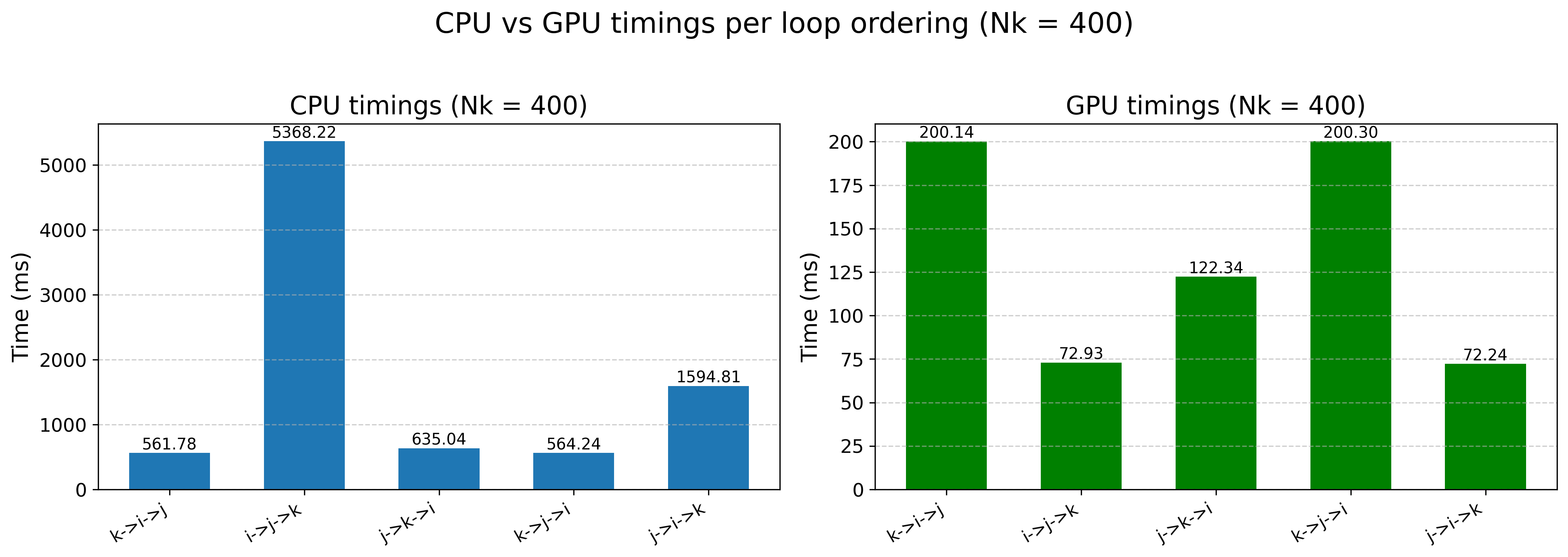
Here you can see a big difference in the timings between the GPU and the CPU code. Plus, if we plot the speedup:
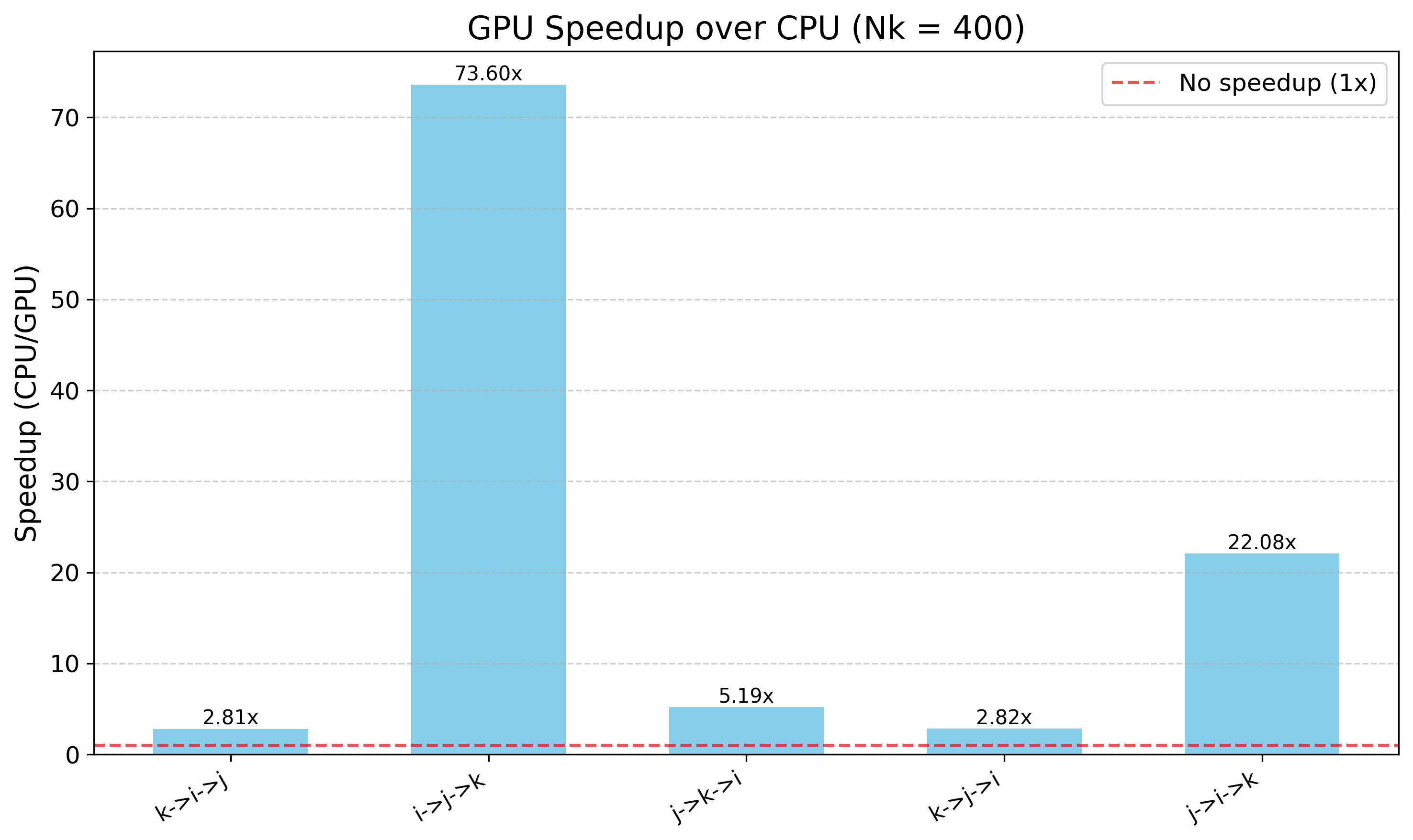
you can see that we get some crazy speedups! But these don’t make much sense if we analyze the first graph correctly.
As we expected, the best loop structure for the CPU might not correlate to the best one for the GPU. This is mostly due to hardware differences between the CPU and the GPU, and how we take advantage of the massive parallelism in the GPU.
You can see that the best loop for the GPU is the j->i->k style, i.e. we loop over all the horizontal plane and then for each point in there we launch the ks serially. Whereas for the CPU, the best loop structure is: k->i->j where we first distribute the vertical layers and then loop over the horizontal ones.
So how does it look if we use the best CPU and the best GPU?
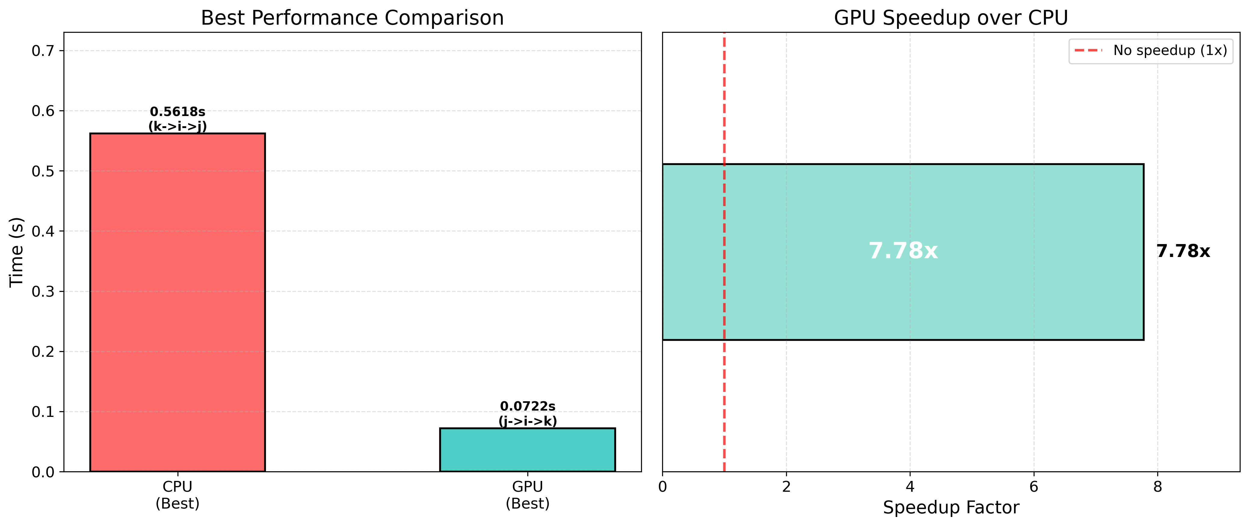
You can see that the speedup is reduced to around 7.78x, which makes a lot more sense. How can we know this? Well, we look at FLOPs.
The V100 has a peak flop rate of 7.7 TFLOP/s, based on the NVIDIA provided datasheets. The XEON has a peak of around 700-900 GFLOP/s depending on the frequency at which the CPU is operating. Let’s settle for something around 850 GFLOP/s. This means that if our code is compute bound the maximum speedup we should get is around 9x, so we’re pushing it here. But…is our code compute bound?
If we look at our code again…
     do concurrent (j=1:ny, i=1:nx, mask(i,j) >= 0.0_real64)
        do k = 2, nz-1
           a_loc   = a3d(i,j,k)
           h_loc   = h3d(i,j,k)
           ray_loc = ray(i,j)
           b1_loc  = b1(i,j)
           d1_loc  = d1(i,j)

           c1(i,j,k) = dt * a_loc * b1_loc

           b_denom = h_loc + dt * (ray_loc + a_loc * d1_loc)
           b1_loc  = one / (b_denom + dt * a3d(i,j,k+1))
           d1_loc  = b_denom * b1_loc

           u_prev  = unew(i,j,k-1)
           u_loc   = (h_loc * u(i,j,k) + dt * a_loc * u_prev) * b1_loc
           unew(i,j,k) = u_loc

           b1(i,j) = b1_loc
           d1(i,j) = d1_loc
        end do
     end do
You can see that it is doing very little FLOPs, 15 to be exact if my counting is not wrong. So we will be spending way more time loading variables from memory, so our kernel is memory bound. So our kernel’s max speedup will be determined by the peak bandwidth of the devices. For the CPU it will be around 60-70 GB/s while for the GPU it should be around 900 GB/s. So the maximum speedup we should be able to get will be around 12-15x. So our 7x speedup is very well within the possibility of what we can do!
So, what happens for the other cases where we see a 73x speedup? Well, for that one we’re comparing the best performing one (the one that favors the memory accesses the most) against one of the worst (not using memory accesses very well). So we’re able to go above the best theoretical speedup because one of our implementations is not using the hardware well.
Memory layouts matter a lot#
Well, we have confirmed that CPUs and GPUs are different, yay. Which means that if you want to parallelize your application using do concurrent in Fortran, you need to check if you’re using the hardware in the best possible fashion. The best way to do this is to think about data locality and how the cache lines are being used.
Another great way to do it is doing something similar to what we did. We created a mini-app which we used to benchmark and compare the performance across the different loop structures.
So let’s look at the problem we’re solving…the key aspect of this problem is that it is based on a tridiagonal solver across the k (vertical) direction. This means that the k loop needs to ALWAYS be processed sequentially, otherwise we get bogus results. So process the entirety of k sequentially per (i,j) column.
In Fortran arrays are in column-major ordering, i.e. here a(i,j,k) the i varies the fastest, then j, then k. So contiguous access along the i direction is optimal. For the CPU:
do k = 1, nk
	do concurrent(i=1:ni, j=1:nj) !or j->i, they are very similar!
This works great because the outer loop is sequential, so for each k, the i,j or j,i loop is collapsed and parallelized across 40 threads on the CPU, each one working on a different (i,j) pair. This has good cache locality, since the inner loops access with a stride-1.
Why is this bad on the GPU? We have nk layers each one having ni*nj points to traverse. So for each k, we have ni*nj work and we have (on the CPU) a limited amount of threads. So on the GPU our only source of parallelism within each slice and we’ve introduced serialization at the k global level! We’re idling waiting for each K to complete.
Now for the GPU:
do concurrent(j=1:nj, i=1:ni)
	do k = 1, nk
Our parallelism is based on the ni*nj number of loop iterations we’d need to do, since the GPU has access to enough threads to launch all of these concurrently we can expose a massive amount of parallelism.
So, why is this bad on the CPU? we’re parallelizing across the ni*nj space. So for realistic sizes, ni*nj > nthreads so we’re limiting the amount of parallelism we can expose. Additionally, the strides between the ks will be very large and lead to cache misses.
These are good things to think about when porting your applications from CPUs to GPUs.
Portability and compile flags#
do concurrent is praised for its portability, similar to OpenMP offloading. One single code to rule them all, it seems (?). Across compilers the support is varied, the best thing to do is to use the compiler the hardware vendor provides. On NVIDIA you use nvfortran, on AMD you use amdflang, and on Intel you use ifx. The key flags you need to be aware of are:
- NVIDIA: `nvfortran -mp=gpu -stdpar=gpu -gpu=mem:separate`
- AMD:    `amdflang -fopenmp --offload-arch=gfx90a -fdo-concurrent-to-openmp=device`
- INTEL:  `ifx -fiopenmp -fopenmp-targets=spir64  -fopenmp-target-do-concurrent  -fopenmp-do-concurrent-maptype-modifier=none`
So, where’s the pudding? See:

This is the benchmark done above but for multiple number of vertical layers. You can see that the PVC is the faster GPU while the V100 and the MI250X are performing quite similarly. The support of do concurrent offloading using the amdflang compiler is quite beta at the moment. I am hoping that in the next couple of months things get better, since the MI250X should be much faster than the V100.
Conclusions#
So, we have done quite a nice benchmark to test how do concurrent works and how portability of the code can be affected between host (multicore) and device plus how do concurrent works on Intel, AMD, and NVIDIA GPUs. We showcased
some of the capabilities of OpenMP to handle memory allocations to minimize memory transfers without depending on the runtime handling arrays.
Additionally, we tested how the distribution and parallelization of the work matters greatly for the device. Sadly, this means that if you want to get the best performance always you’ll need to constantly benchmark the code and/or write different kernels for each type of device you use.
I hope this is of use for people who want to explore Fortran to enable GPU acceleration in your workloads without having to learn C,C++. Next up, calling CUDA kernels from Fortran. Because yes, you can still use openmp to handle memory and launch cuda kernels.